When you are developing your model, you want to be able to quickly execute code, see outputs, and make iterative improvements. Domino enables this with Workspaces. Step 3 covered starting a Workspace and explored Workspace options like VSCode, RStudio, and Jupyter.

In this section, we will use Jupyter to load, explore, and transform some data. After the data has been prepared, we will train a model.

Step 5.1: Load and explore the dataset

From the project menu, click Workspaces.
Click Open Last Workspace or Open in the workspace created in Step 3. In /mnt, you can see data.csv. If not, go to Step 4 to download the dataset.
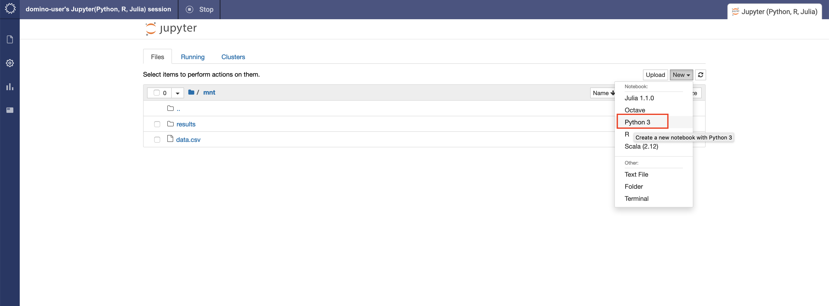
Use the New menu to create a Python notebook.
Starting in the first cell, enter these lines to import some packages. After each line, press Shift+Enter to execute:
```
%matplotlib inline
import pandas as pd
import datetime
```

Next, read the file you downloaded into a pandas dataframe:

df = pd.read_csv('data.csv', skiprows=1, skipfooter=1, header=None, engine='python')

Rename the columns according to information on the column headers at https://www.bmreports.com/bmrs/?q=generation/fueltype/current and display the first five rows of the dataset using df.head().
```
df.columns = ['HDF', 'date', 'half_hour_increment',
              'CCGT', 'OIL', 'COAL', 'NUCLEAR',
              'WIND', 'PS', 'NPSHYD', 'OCGT',
              'OTHER', 'INTFR', 'INTIRL', 'INTNED',
               'INTEW', 'BIOMASS', 'INTEM','INTEL',
               'INTIFA2', 'INTNSL']
df.head()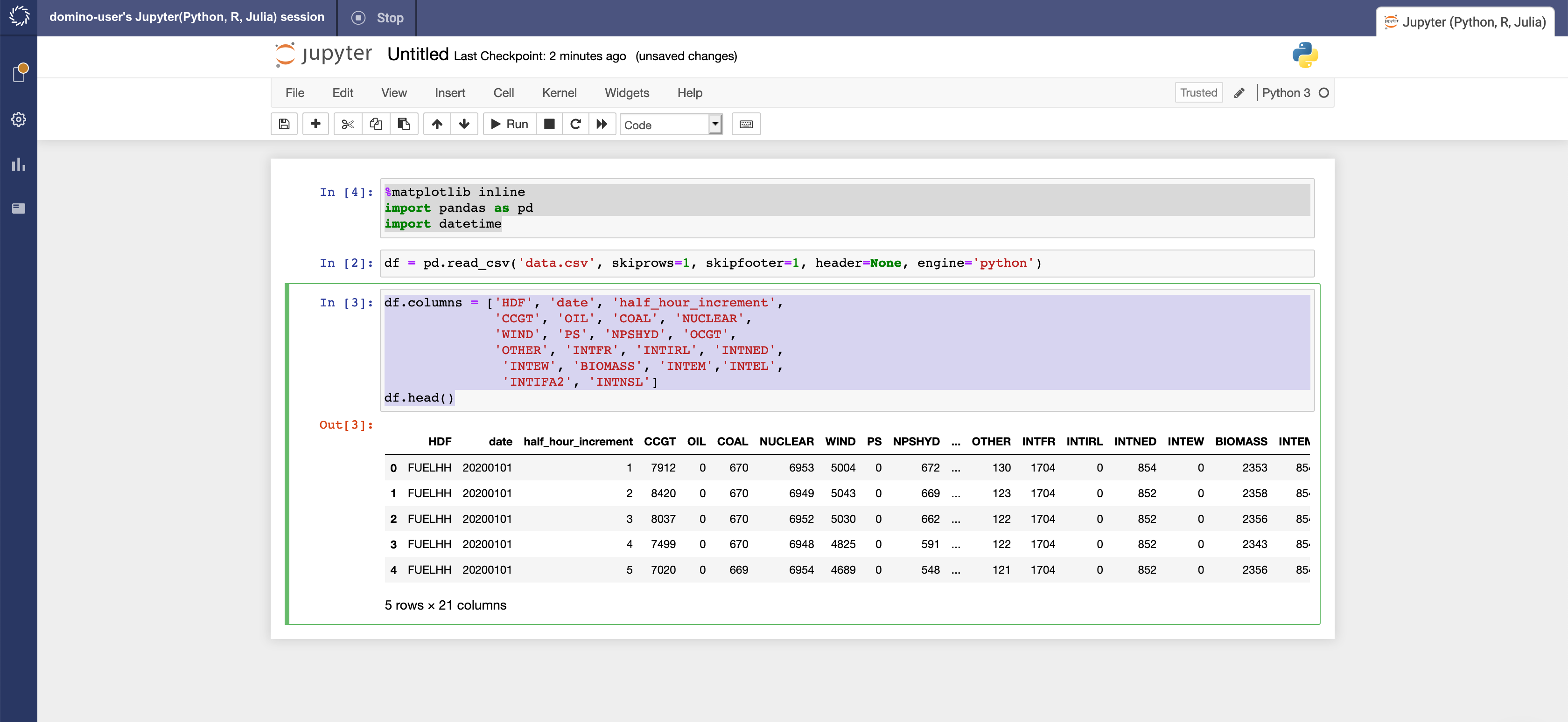
```
We can see that this is a time series dataset. Each row is a successive half hour increment during the day that details the amount of energy generated by fuel type. Time is specified by the date and half_hour_increment columns.
Create a new column named datetime that represents the starting datetime of the measured increment. For example, a 20190930 date and 2 half hour increment means that the time period specified is September 19, 2019 from 12:30am to 12:59am.
```
df['datetime'] = pd.to_datetime(df['date'], format="%Y%m%d")
df['datetime'] = df.apply(lambda x:x['datetime']+ datetime.timedelta(minutes=30*(int(x['half_hour_increment'])-1)), axis = 1)
```
Visualize the data to see how each fuel type is used during the day by plotting the data.
```
df.drop(
    ['HDF', 'date', 'half_hour_increment'], axis = 1
    ).set_index('datetime').plot(figsize=(15,8))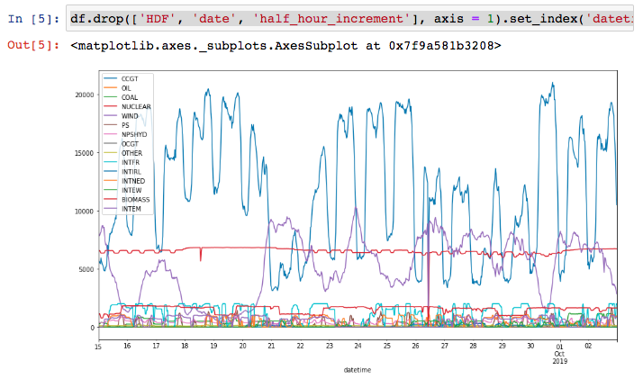
```
The CCGT column, representing combined-cycle gas turbines, generates a lot of energy and is volatile.

We will concentrate on this column and try to predict the power generation from this fuel source.

Step 5.2: Train a model

Data scientists have access to many libraries and packages that help with model development. Some of the most common for Python are XGBoost, Keras and scikit-learn. These packages are already installed in the Domino Analytics Distribution (DAD), . However, there might be times when you want to experiment with a package that is not installed in the environment.

We will build a model with the Facebook Prophet package, which is not installed into the default environment. You will see that you can quickly get started with new packages and algorithms just as fast as they are released into the open source community.

In the next Jupyter cell, install Facebook Prophet and its dependencies, including PyStan (a slightly older version of Plotly, which is compatible with Prophet), and Cufflinks. PyStan requires 4 GB of RAM to be installed. Make sure your workspace is set to use a large enough hardware tier:
```
!pip install cufflinks==0.16.0
!sudo -H pip install -q --disable-pip-version-check "pystan==2.17.1.0" "plotly<4.0.0"
!pip install -qqq --disable-pip-version-check fbprophet==0.6
```
For Facebook Prophet, the time series data needs to be in a DataFrame with 2 columns named ds and y:
```
df_for_prophet = df[['datetime', 'CCGT']].rename(columns = {'datetime':'ds', 'CCGT':'y'})
```

Split the dataset into train and test sets:

X = df_for_prophet.copy()
y = df_for_prophet['y']
proportion_in_training = 0.8
split_index = int(proportion_in_training*len(y))
X_train, y_train = X.iloc[:split_index], y.iloc[:split_index]
X_test, y_test = X.iloc[split_index:], y.iloc[split_index:]

Import Facebook Prophet and fit a model:
```
from fbprophet import Prophet
m = Prophet()
m.fit(X_train)
```
If you encounter an error when running this cell, you may need to downgrade your pandas version first. In that case you would run
```
!sudo pip install pandas==0.23.4
```
and then
```
from fbprophet import Prophet
m = Prophet()
m.fit(X_train)
```
After running the code above, you may encounter a warning about code deprecation. The warning can be ignored for the purposes of this walkthrough.

Make a DataFrame to hold prediction and predict future values of CCGT power generation:

future = m.make_future_dataframe(periods=int(len(y_test)/2), freq='H')
forecast = m.predict(future)
# forecast[['ds', 'yhat', 'yhat_lower', 'yhat_upper']].tail() #uncomment to inspect the DataFrame

Plot the fitted line with the training and test data:

import matplotlib.pyplot as plt
plt.gcf()
fig = m.plot(forecast)
plt.plot(X_test['ds'].dt.to_pydatetime(), X_test['y'], 'r', linewidth = 1, linestyle = '--', label = 'real')
plt.legend()

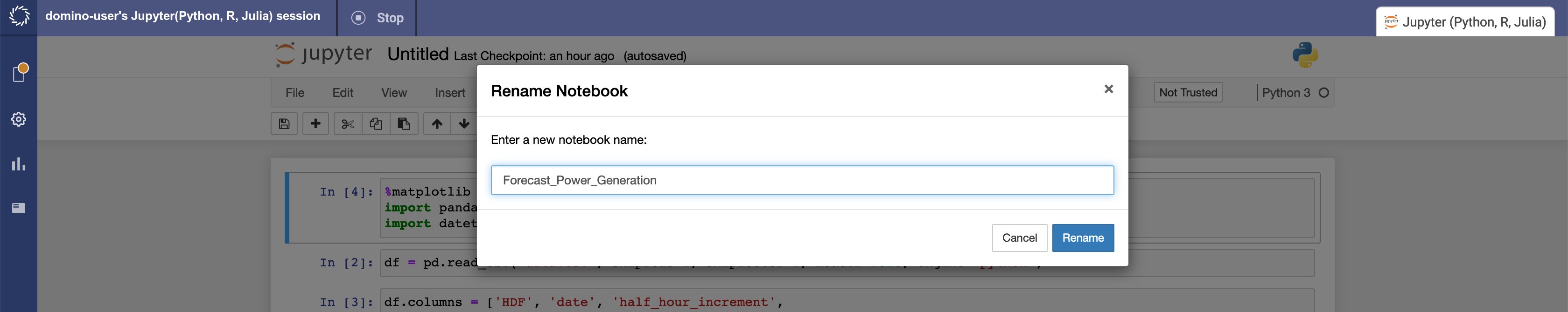
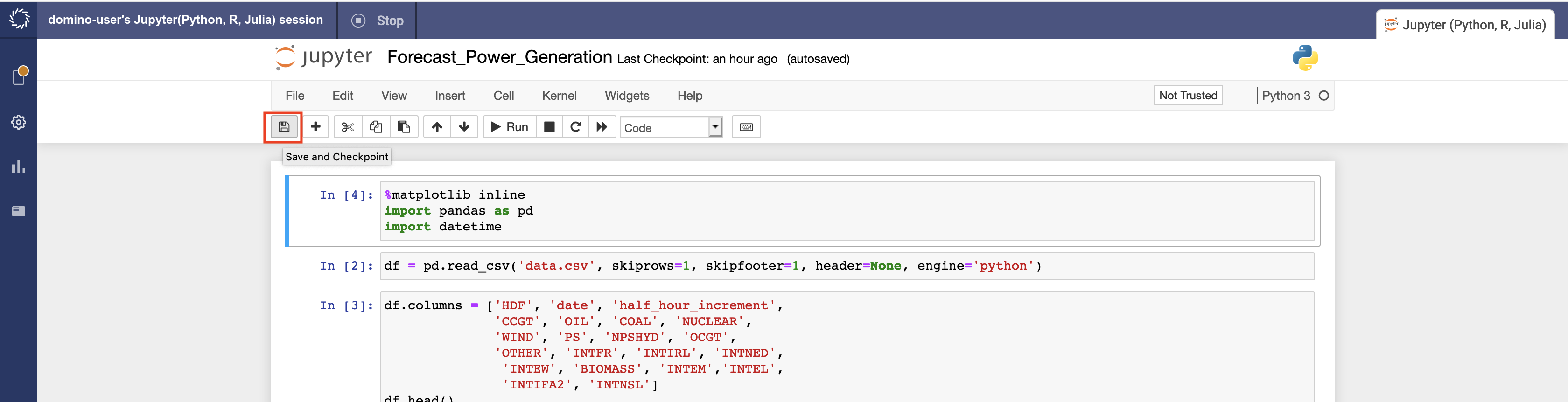
Rename the notebook to be Forecast_Power_Generation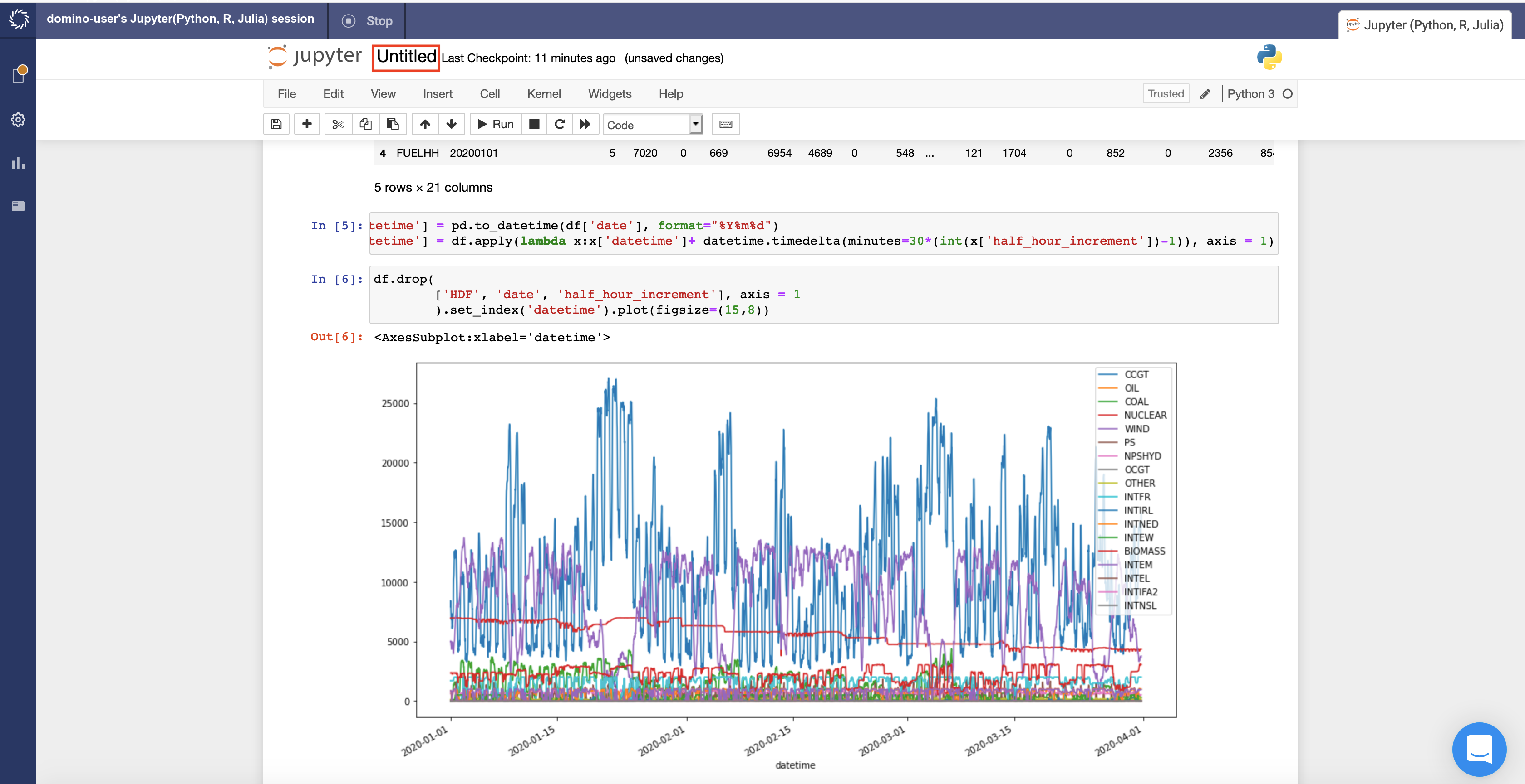
Save the notebook.

Step 5.3: Export the model

Trained models are meant to be used. There is no reason to re-train the model each time you use the model. Export or serialize the model to a file to load and reuse the model later. In Python, the pickle module implements protocols for serializing and de-serializing objects. In R, you can commonly use the serialize command to create RDS files.

Export the trained model as a pickle file for later use:

import pickle
# m.stan_backend.logger = None    #uncomment if using Python 3.6 and fbprophet==0.6
with open("model.pkl", "wb") as f:
      pickle.dump(m, f)

We will use the serialized model in Step 7 when we create an API from the model.

Step 5: Develop your model

Step 5.1: Load and explore the dataset

Step 5.2: Train a model

Step 5.3: Export the model